Understand the Goal, Advantages/ Disadvantages, and practical Implementation of Decision Trees.
Decision Trees are non-parametric supervised machine learning algorithm that can be used for classification (when the target is categorical), Regression (When the target is numerical), and also for subjective segmentation.
Non- parametric means non-mathematical i.e., there is no estimation happening in the backend (e.g., Ordinary list Square Estimation in Linear Regression). A decision tree creates a model that predicts the target variable by learning simple rules inferred from the data features. The deeper the tree, the more complex the decision rules, and the fitter the model.
Some Advantages:
- Simple to understand, interpret, and visualize
- Required very little data preparation
- Performs well even if its assumptions are somewhat violated by the actual model from which the data were generated
Some Disadvantages:
- It can create over-complex trees that do not generalize the data well This is called overfitting. Mechanisms such as pruning, setting the minimum number of samples required at a leaf node, or setting the maximum depth of the tree are necessary to avoid this problem.
- It can be unstable because of small variations in data might result in a completely different tree being generated. This can be mitigated by using decision trees within an ensemble, which we see in my upcoming blog.
- Predictions of decision trees are neither smooth nor continuous, but piecewise constant approximations, Therefore, they are not good at extrapolation.
- If some classes dominate the Decision tree learners can create biased trees. Therefore, it is recommended to balance the dataset before fitting it with the decision tree.
Some Important Terminologies:
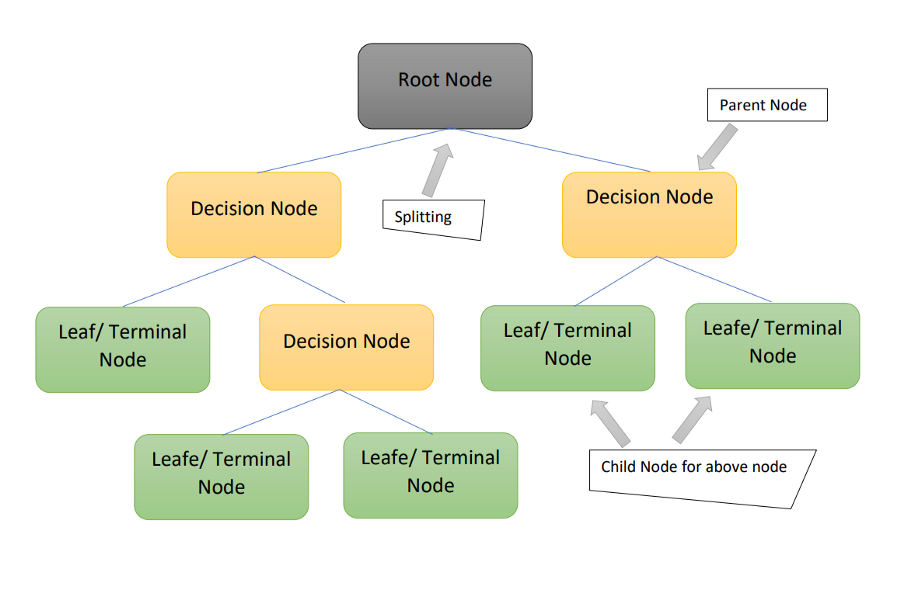
- Root Node: It represents the entire population or sample, and this further gets divided into two or more homogeneous sets
- Decision Node: When a sub-node splits into further sub-nodes, then it is called the decision node.
- Leaf / Terminal Node: Nodes that do not split are called Leaf or Terminal nodes.
- Splitting: It is a process of dividing a node into two or more sub-nodes.
- Parent and Child Node: A node, which is divided into sub-nodes is called a parent node of sub-nodes whereas sub-nodes are the child of a parent node.
- Branch / Sub-Tree: A subsection of the entire tree is called a branch or sub-tree.

Let’s train and visualize a decision tree:
lets us build one decision tree and take a look at the path our algorithm went through to make a particular prediction. In this article, we will be using the famous iris dataset for explanation purposes.
Training Steps
1. Let’s import the iris dataset from sklearn.datasets and our decision tree classifier from sklearn.tree
from sklearn.datasets import load_iris
from sklearn import tree
2. Let’s Separate out features (X) and target (y) for the training
iris = load_iris()
X, y = iris.data, iris.target
3. Let’s Initializing a decision tree classifier with max_depth=2
clf = tree.DecisionTreeClassifier(max_depth=2)
clf = clf.fit(X, y)
Keeping Max depth 2, so it will be easy to visualize how decisions are made in the decision tree. Keeping all other hyperparameters default.
Visualizing Tree
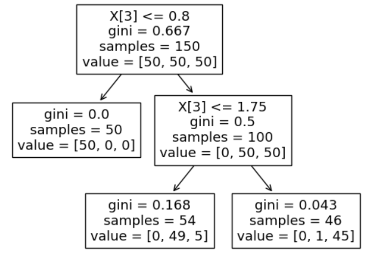
Once trained, you can plot the tree with the plot_tree function:
tree.plot_tree(clf)
Visualizing With Graphviz
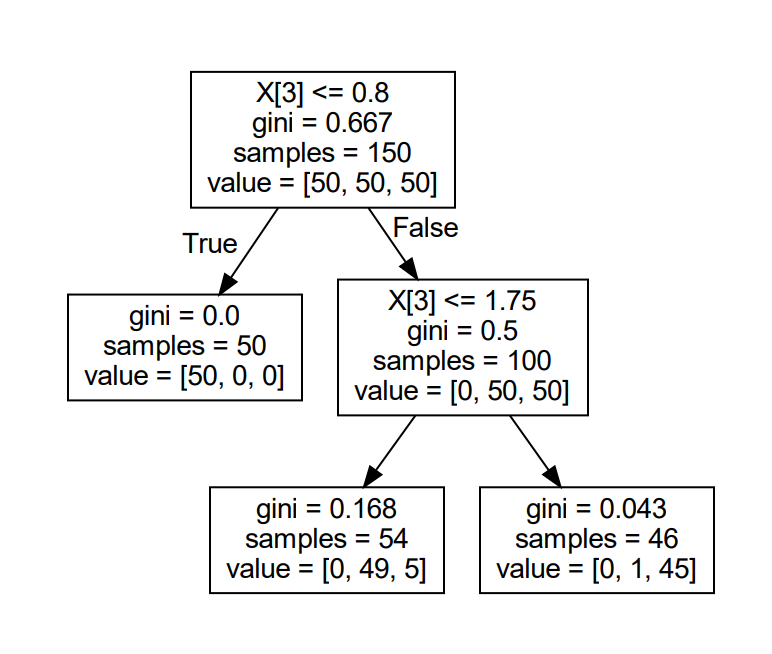
We can also export the tree in Graphviz format using the export_graphviz exporter. (Note Python wrapper installed from pypi with pip install graphviz), Below is an example graphviz export of the above tree trained on the entire iris dataset; the results are saved in an output file iris.pdf
import graphviz
dot_data = tree.export_graphviz(clf, out_file=None)
graph = graphviz.Source(dot_data)
graph.render("iris") 
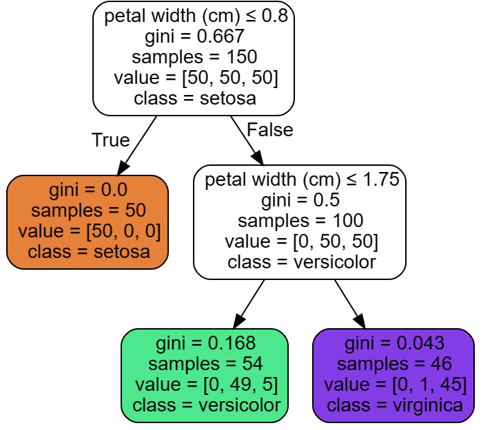
epport_graphviz also supports a variety of options, including coloring nodes by their class (or value in regression) and using explicit variables and class names if desired. Jupyter notebooks also render these plots inline automatically:
dot_data = tree.export_graphviz(clf, out_file=None,
                      feature_names=iris.feature_names,
                      class_names=iris.target_names,
                      filled=True, rounded=True,
                      special_characters=True)
graph = graphviz.Source(dot_data)
graph
Awesome as you can see above we have beautiful looking visualization of our tree. Let us understand what it has to tell us.
As we can see petal width has been chosen as the root node.
Is petal width(cm) <= 0.8?
If Yes/ True –> Then the class assigned (Prediction) is setosa
If No/ False –> Then the The Next Question DT asked, is petal width(cm) <=1.75
If Yes/ True –> Then the class assigned (Prediction) is versicolor
If No/ False –> Else Prediction is virginica
This is how a series of if-else questions are asked to the rich the final prediction or this is how decisions are made in the Decision Tree
Important Hyperparameters
max_depth : int, default=None
The maximum depth of the tree. If None, then nodes are expanded until all leaves are pure or until all leaves contain less than min_samples_split samples.
This is a very important parameter as with a higher value (or default value) we end up with a highly complex (high variance decision tree), And with a very lower value, we will have a highly biased tree.
min_samples_split: int or float, default=2
The minimum number of samples required to split an internal node.
with a low value (or default value) we will end up with a highly complex (high variance decision tree), And with a very higher value, we will have a highly biased tree.
min_samples_leaf: int or float, default=1
A minimum number of samples is required to be at a leaf node. A split point at any depth will only be considered if it leaves at least min_samples_leaf training samples in each of the left and right branches.
ccp_alpha: non-negative float, default=0.0
Complexity parameter used for Minimal Cost-Complexity Pruning. The subtree with the largest cost complexity that is smaller than ccp_alpha will be chosen. By default, no pruning is performed.
Conclusion
Congratulations!
We have just trained and visualized one of the simple but very important machine learning algorithm with some important fundamentals. decision trees are really easy to use, understand and interpret. But the issue with decision trees is that they are extremely sensitive to minor variations in the training data. Issues in the Decision Tree can be countered by using Random Forests which we will be discussing in the upcoming blogs. Stay tuned!!
Hope this article help fellow Data Scientist and aspirants
Thanks for reading this article! leave a comment 💬! and stay tuned to new articles on Data Science and Statistics.


Great Work